The Kruskal-Wallis test, derived from first principles

Deriving the Kruskal-Wallis test from scratch, using a pain management trial to show where ANOVA falls short.

Let’s say that we want to test the effects of pain management protocols. We have 45 post-surgical patients randomized to three groups: opioid-only, NSAID + nerve block and multimodal. 48 hours after their operations, each patient marks their pain on a 0–10 visual analog scale (VAS). The question that the clinic is interested in is whether the three different protocols produce different pain levels or not.

ANOVA [1] is a popular test for testing whether group means are equal. The problem with ANOVA in the pain scale example is that the pain scores are typically right-skewed (clustering around 2-4) and with small sample sizes, the within-group variance can be inflated by some observations being at the right tail (8-10). ANOVA computes an F-statistic as a ratio of between-group variance to within-group variance. If the within group variance is inflated, ANOVA needs a larger between-group variance to detect a difference.

The Kruskal-Wallis test solves this problem. The KW test replaces raw scores with their ranks in the pooled dataset (see Figure 2) and tests whether the ranks cluster by treatment. Under the null hypothesis, the ranks should equally be distributed to the groups.

NoteNotation used in this post

Symbol	Meaning
K	Number of groups
j	Group index, j \in \{1, \ldots, K\}
n_j	Number of observations in group j
N	Total sample size N = \sum_j n_j
x_{ij}	The i-th observation in group j
R_{ij}	Rank of x_{ij} among all N pooled observations
R_j	Rank sum of group j: R_j = \sum_i R_{ij}
\bar{R}_j	Mean rank of group j: \bar{R}_j = R_j / n_j
\bar{R}	Grand mean rank: \bar{R} = (N+1)/2
H	Kruskal-Wallis test statistic
F	ANOVA F-statistic
\chi^2(K-1)	Chi-square distribution with K-1 degrees of freedom

The pain trial

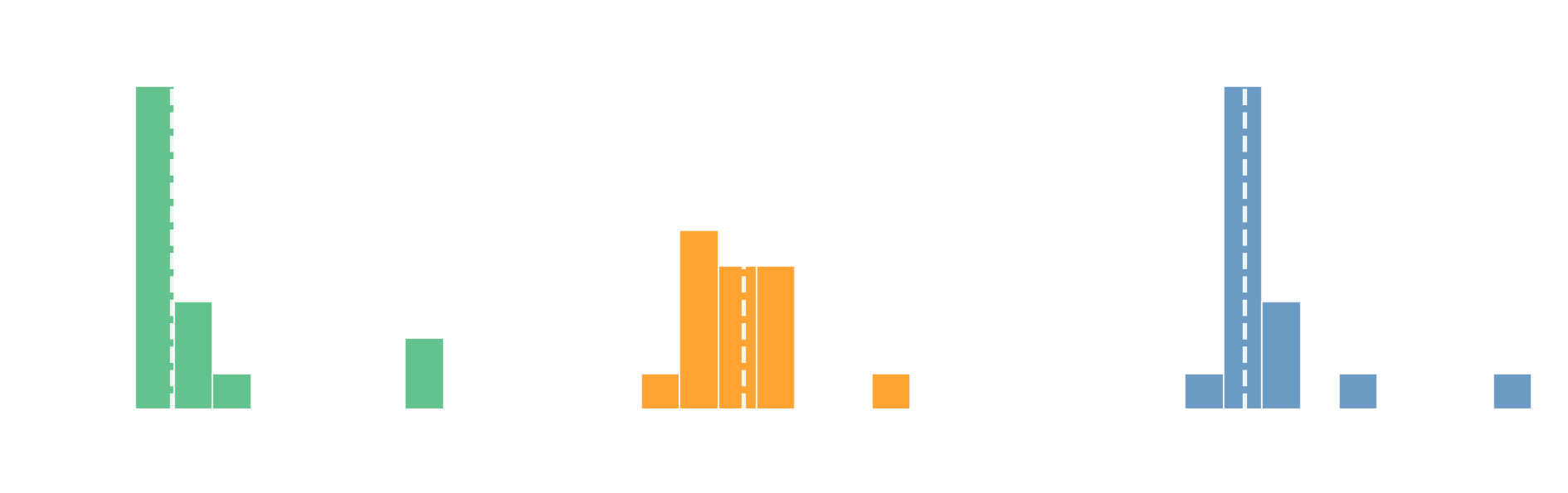
This post will use a made up example: the data will have three groups of 15 patients with NRS scores at 48 hours post surgery. The Figure 1 shows both the theoretical (Gamma) distributions where the samples are drawn from and the actual samples. Then Table 1 summarizes the data.

import numpy as np
import matplotlib.pyplot as plt
from scipy import stats

# VAS pain scores at 48 h post-op (0 = no pain, 10 = worst imaginable)
# Gamma(shape=0.5) → heavy right skew; offset shifts group medians apart
rng = np.random.default_rng(99)
pain_a = np.clip(np.round(rng.gamma(0.5, 3.0, 15) + 1.0, 2), 0, 10)  # multimodal:          mean ≈ 2.6
pain_b = np.clip(np.round(rng.gamma(0.5, 3.0, 15) + 1.8, 2), 0, 10)  # NSAID + nerve block: mean ≈ 3.4
pain_c = np.clip(np.round(rng.gamma(0.5, 3.0, 15) + 2.6, 2), 0, 10)  # opioid-only:         mean ≈ 3.9

labels = ["Multimodal", "NSAID + nerve block", "Opioid-only"]
colors = ["mediumseagreen", "darkorange", "steelblue"]
groups = [pain_a, pain_b, pain_c]

plt.rcParams.update(
    {
        "text.color": "white",
        "axes.labelcolor": "white",
        "xtick.color": "white",
        "ytick.color": "white",
        "axes.edgecolor": "white",
    }
)

fig, axes = plt.subplots(1, 3, figsize=(10, 3.2), sharey=True, sharex=True)
fig.patch.set_alpha(0)

for ax, g, color, label in zip(axes, groups, colors, labels):
    ax.hist(
        g,
        bins=np.linspace(0, 10, 12),
        color=color,
        alpha=0.8,
        edgecolor="white",
        linewidth=0.8,
    )
    ax.axvline(np.median(g), color="white", linewidth=2, linestyle="--", alpha=0.9)
    ax.set_title(f"{label}\nmedian = {np.median(g):.1f}", fontsize=10, color="white")
    ax.set_xlabel("Pain score (0–10)")
    ax.set_xlim(-0.5, 10.5)
    ax.patch.set_alpha(0)

axes[0].set_ylabel("Count")
plt.tight_layout()
plt.show()

Figure 1: VAS pain scores at 48 h post-surgery for three protocols. Dashed line shows the group median.

from IPython.display import HTML

rows = "".join(
    f"<tr><td style='padding:5px 14px;'>{lbl}</td>"
    f"<td style='padding:5px 14px; text-align:right;'>{len(g)}</td>"
    f"<td style='padding:5px 14px; text-align:right;'>{g.mean():.2f}</td>"
    f"<td style='padding:5px 14px; text-align:right;'>{np.median(g):.1f}</td>"
    f"<td style='padding:5px 14px; text-align:right;'>{g.std(ddof=1):.2f}</td></tr>"
    for lbl, g in zip(labels, groups)
)
th = "padding:6px 14px; text-align:right; border-bottom:1px solid #555;"
th_l = "padding:6px 14px; text-align:left; border-bottom:1px solid #555;"
display(HTML(f"""
<table style="border-collapse:collapse; font-size:0.9em;">
  <thead><tr>
    <th style="{th_l}">Protocol</th>
    <th style="{th}">n</th>
    <th style="{th}">Mean</th>
    <th style="{th}">Median</th>
    <th style="{th}">SD</th>
  </tr></thead>
  <tbody>{rows}</tbody>
</table>
"""))

Table 1: Summary statistics for the three pain management protocols.

Protocol	n	Mean	Median	SD
Multimodal	15	2.57	1.8	2.21
NSAID + nerve block	15	3.21	3.3	1.37
Opioid-only	15	3.93	3.2	1.92

The key insight: order is enough

For deducing whether one protocol produces less pain than another, we don’t need to know how much less. We only need to know who ranks lower. Thus we use a ranking transformation. The animation in Figure 2 shows how the data points are transformed into ranks.

viewof transform_t = Inputs.range(
  [0, 1],
  { step: 0.005, value: 0, label: "← original values  ·  ranks →" }
)

rt_colors = ["steelblue", "darkorange", "mediumseagreen"]
N_rt = pain_groups.flat().length

rt_flat_pain = pain_groups.flatMap((g, j) => g.map(v => ({ v, group: j })))

rt_ranks_pain = (() => {
  const indexed = rt_flat_pain.map((d, i) => ({ v: d.v, i })).sort((a, b) => a.v - b.v);
  const ranks = new Array(rt_flat_pain.length);
  let i = 0;
  while (i < indexed.length) {
    let j = i;
    while (j < indexed.length - 1 && indexed[j + 1].v === indexed[j].v) j++;
    const avg = (i + j) / 2 + 1;
    for (let k = i; k <= j; k++) ranks[indexed[k].i] = avg;
    i = j + 1;
  }
  return ranks;
})()

rt_x_lo = (1 - transform_t) * 0  + transform_t * 1
rt_x_hi = (1 - transform_t) * 10 + transform_t * N_rt

rt_pts_groups = rt_flat_pain.map((d, i) => ({
  x: (1 - transform_t) * d.v + transform_t * rt_ranks_pain[i],
  y: pain_labels[d.group],
  group: pain_labels[d.group],
}))

rt_pts_pooled = rt_flat_pain.map((d, i) => ({
  x: rt_ranks_pain[i],
  y: "Pooled",
  group: pain_labels[d.group],
}))

Plot.plot({
  width: 680,
  height: 270,
  marginLeft: 145,
  marginRight: 20,
  x: {
    label: transform_t < 0.05 ? "Pain score (0–10) →"
         : transform_t > 0.95 ? `Rank (1–${N_rt}) →`
         : "Transforming… →",
    domain: [rt_x_lo, rt_x_hi],
  },
  y: {
    domain: [...pain_labels, "Pooled"],
    label: null,
  },
  color: {
    domain: pain_labels,
    range: rt_colors,
  },
  marks: [
    Plot.dot(rt_pts_groups, {
      x: "x", y: "y",
      fill: "group", r: 7,
      fillOpacity: 0.85,
      stroke: "white", strokeWidth: 0.8,
    }),
    Plot.dot(rt_pts_pooled, {
      x: "x", y: "y",
      fill: "group", r: 7,
      fillOpacity: transform_t * 0.85,
      stroke: "white", strokeWidth: 0.8,
      strokeOpacity: transform_t,
    }),
  ],
})

Figure 2: Each dot is one of the 45 patients, coloured by protocol. Drag to 1: each pain score is replaced by its rank in the pooled dataset, spreading the dots uniformly. The pooled row fades in to show all 45 ranks in sequence.

Deriving the H statistic

Setting up the problem

Abstracting from the medical example, let’s say that we have K groups with the number of observations in each group being n_1, ..., n_K. Then the total number of observations is N = \sum_j n_j. After combining the observations into one pool and ranking them (as shown in Figure 2), let R_{ij} be the rank of the i-th observation in group j.

The goal is to test whether the groups share the same distribution with each other. Transforming this into a null hypothesis becomes

H_0: \text{the ranks } 1, 2, \ldots, N \text{ are randomly distributed across groups}

So the next question to answer is: what does a large deviation from the random distribution look like and how can we measure the deviation?

Expected rank mean under H_0

Under H_0, every rank is equally likely to fall into any group. Then the expected value of a single rank R drawn from the uniform set \{1, \ldots, N\} is

\mathbb{E}[R] = \frac{1}{N} \sum_{r=1}^{N} r = \frac{1}{N}\frac{N(N+1)}{2} = \frac{N+1}{2} \tag{1}

The expected mean rank in all groups is \bar{R} = \frac{N+1}{2}, regardless of the individual group sizes. The only thing that matters is the total sample size. If H_0 is true, all groups’ mean ranks should hover around \bar{R}.

Building the test statistic

A natural way to measure deviation from the null is the squared distance of each group’s mean rank \bar{R}_j from the expected grand mean:

T = \sum_{j=1}^{K} n_j \left(\bar{R}_j - \frac{N+1}{2}\right)^2 \tag{2}

Here n_j is the size of group j to weight the penalty of bigger groups more because we have more information of them. This structure is extremely similar to ANOVA that is defined as the between group sum of squared deviations from each group mean from the global mean:

SS_{\text{between}} = \sum_{j=1}^{K} n_j \left(\bar{x}_j - \bar{x}\right)^2

The 12/N(N+1) scaling factor

To turn T from Equation 2 into a statistic with a known null distribution, we need to normalize it by the variance of the ranks. With Equation 1, the variance for a discrete uniform distribution on \{1, \dots, N\} is:

\begin{align*} \text{Var}(R) = \sigma^2_R &= \mathbb{E}[R^2] - \left(\mathbb{E}[R]\right)^2 \\ &= \frac{1}{N}\sum_{r=1}^{N} r^2 - \left(\frac{N+1}{2}\right)^2 \\ &= \frac{(N+1)(2N+1)}{6} - \frac{(N+1)^2}{4} \\ &= (N+1)\left[\frac{2(2N+1)}{12} - \frac{3(N+1)}{12}\right] \\ &= (N+1) \cdot \frac{4N+2 - 3N-3}{12} \\ &= \frac{(N+1)(N-1)}{12} \\ &= \frac{N^2-1}{12} \end{align*}

By analogy with the ANOVA F-statistic, we normalise T by SS_{\text{total}}/(N-1), where the total rank sum-of-squares for the complete set of ranks \{1,\dots,N\} is SS_{\text{total}} = N\sigma^2_R = \frac{N(N^2-1)}{12}:

H = (N-1)\cdot\frac{T}{SS_{\text{total}}} = \frac{12}{N(N+1)} \sum_{j=1}^{K} n_j \left(\bar{R}_j - \frac{N+1}{2}\right)^2

The factor 12/[N(N+1)] scales H so that its expected value under H_0 equals K-1, which is exactly the degrees-of-freedom parameter of a chi-square distribution. For large N, H \xrightarrow{d} \chi^2(K-1) under H_0.

Back to the pain trial

Now that we’ve shown the mathematical difference between ANOVA and the Kruskal-Wallis test, we can compute the p-values using both of the tests and compare them.

import numpy as np
from scipy import stats

N = sum(len(g) for g in groups)
K = len(groups)

all_scores = np.concatenate(groups)
ranks = stats.rankdata(all_scores)

idx = 0
rank_groups = []
for g in groups:
    rank_groups.append(ranks[idx : idx + len(g)])
    idx += len(g)

grand_mean_rank = (N + 1) / 2
H, p_kw = stats.kruskal(*groups)
F, p_anova = stats.f_oneway(*groups)

from IPython.display import HTML

th = "padding:6px 14px; text-align:right; border-bottom:1px solid #555;"
th_l = "padding:6px 14px; text-align:left; border-bottom:1px solid #555;"
td = "padding:5px 14px; text-align:right;"
td_l = "padding:5px 14px;"

rank_rows = "".join(
    f"<tr><td style='{td_l}'>{lbl}</td>"
    f"<td style='{td}'>{rg.sum():.0f}</td>"
    f"<td style='{td}'>{rg.mean():.2f}</td>"
    f"<td style='{td}'>{rg.mean() - grand_mean_rank:+.2f}</td></tr>"
    for lbl, rg in zip(labels, rank_groups)
)

test_rows = (
    f"<tr><td style='{td_l}'>Kruskal-Wallis</td>"
    f"<td style='{td}'>H = {H:.3f}</td>"
    f"<td style='{td}'>{K - 1}</td>"
    f"<td style='{td}'>{p_kw:.4f}</td></tr>"
    f"<tr><td style='{td_l}'>ANOVA</td>"
    f"<td style='{td}'>F = {F:.3f}</td>"
    f"<td style='{td}'>{K - 1}</td>"
    f"<td style='{td}'>{p_anova:.4f}</td></tr>"
)

display(HTML(f"""
<p style="font-size:0.85em;color:#aaa;margin-bottom:4px;">
  Grand mean rank (null expectation): {grand_mean_rank:.1f}
</p>
<table style="border-collapse:collapse;font-size:0.9em;margin-bottom:1.2em;">
  <thead><tr>
    <th style="{th_l}">Protocol</th>
    <th style="{th}">Rank sum</th>
    <th style="{th}">Mean rank</th>
    <th style="{th}">Deviation</th>
  </tr></thead>
  <tbody>{rank_rows}</tbody>
</table>
<table style="border-collapse:collapse;font-size:0.9em;">
  <thead><tr>
    <th style="{th_l}">Test</th>
    <th style="{th}">Statistic</th>
    <th style="{th}">df</th>
    <th style="{th}">p-value</th>
  </tr></thead>
  <tbody>{test_rows}</tbody>
</table>
"""))

Grand mean rank (null expectation): 23.0

Protocol	Rank sum	Mean rank	Deviation
Multimodal	212	14.17	-8.83
NSAID + nerve block	378	25.20	+2.20
Opioid-only	444	29.63	+6.63

Test	Statistic	df	p-value
Kruskal-Wallis	H = 11.034	2	0.0040
ANOVA	F = 1.976	2	0.1513

The multimodal group’s mean rank is well below 23.0 (the grand mean rank), the opioid-only group’s mean rank is well above it. The NSAID + nerve block is quite close to the mean rank. The H-statistic is able to quantify the spread. The chi-square p-value tells us whether a deviation this large would occur by chance under the null. With p < 0.05, we reject. The KW-test rejects the null, ANOVA doesn’t. This shows that the KW-test is able to quantify the differences between distributions when they are heavily skewed better than ANOVA.

NoteWhat KW doesn’t tell

A statistically significant KW result only says that something differs, not which pairs differ. To investigate which pairs differ, the Dunn test [2] fits this problem well.

References

[1]

Wikipedia contributors, “Analysis of variance.” https://en.wikipedia.org/wiki/Analysis_of_variance, 2025.

[2]

Z. Bobbitt, “Dunn’s test for multiple comparisons.” https://www.statology.org/dunns-test/, 2020.