The Fourier Transform
signal processing
How mathematics hears which notes are hidden in a chord.
An instrument plays three notes at once, but you hear a single chord. Physically, all three notes create pressure waves that sum together and hit your eardrum as one. Your brain is somehow able to recognize the three distinct frequencies hidden in that single wave. The mechanism behind how the brain does this is an extremely complicated topic, but getting machines to decompose the signal is quite straightforward, and this post explains how it is done. The core mathematical operation doing signal decomposition is called the Fourier Transform.
Sound is a sum of sinusoids
A pure tone (a tuning fork or a whistle) is a sinusoid. A sinusoid is a smooth, repetitive oscillation at a single frequency. If you stack multiple pure tones on top of each other, you get a chord. The sounds you hear in your ear on a daily basis are typically a sum of hundreds of pure tones. When looking at the waveforms of chords, it looks like pure noise (see Figure 1), but it isn’t noise. The pure tones are just hiding in the sum of frequencies of the chord signal.
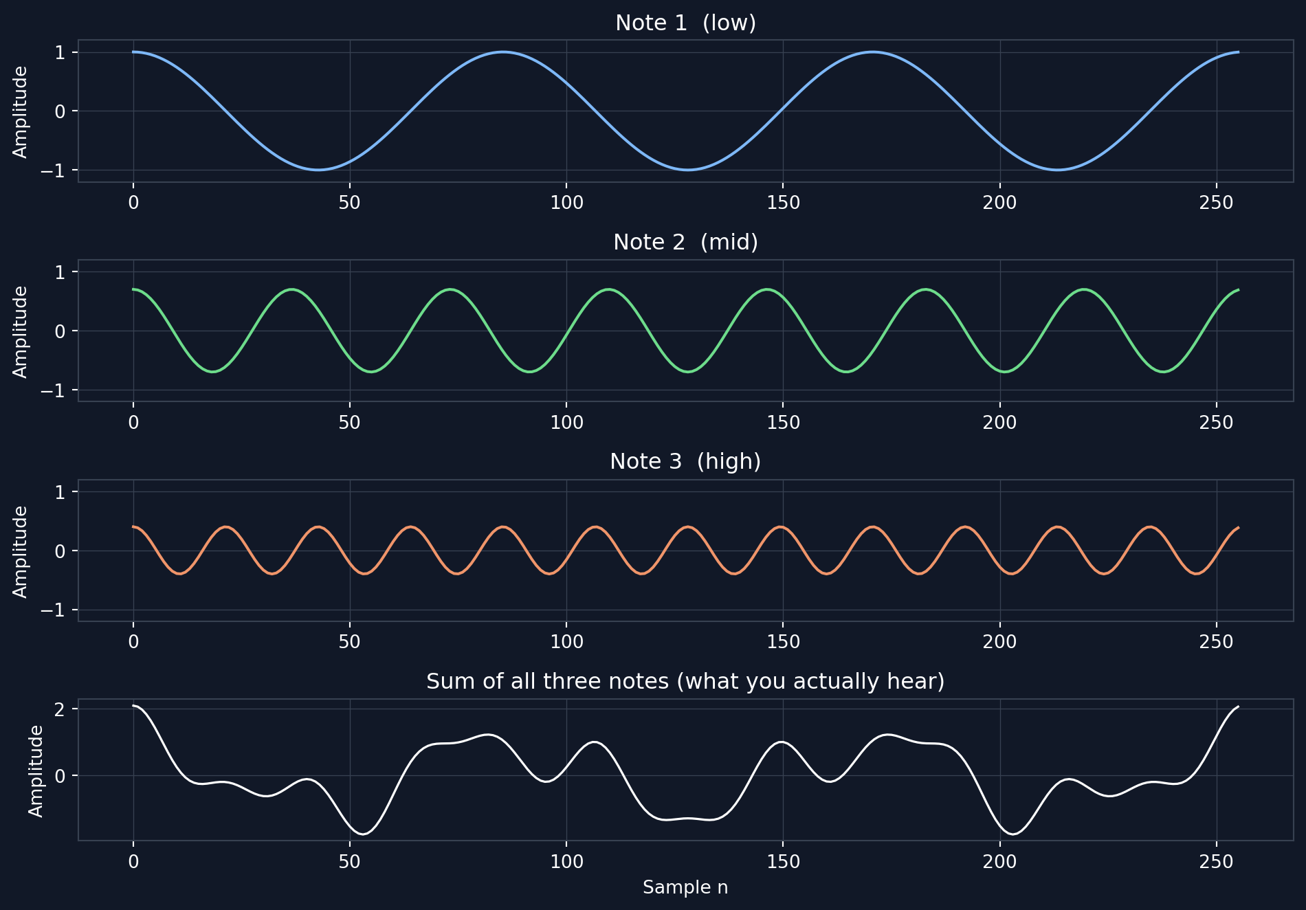
Below you can hear three different pure tones and the chord they produce when combined. Then below the media players, you can see the wave forms of the signals individually and then the signal that is produced when combining the three pure tones.
fs = 8000
t = np.linspace(0, 1.5, int(fs * 1.5), endpoint=False)
note_freqs = [300, 700, 1200]  # Hz ratio 3:7:12, matching the figure below
note_amps = [1.0, 0.7, 0.4]
chord = sum(a * np.cos(2 * np.pi * f * t) for f, a in zip(note_freqs, note_amps))
Note 1 (low)
Note 2 (mid)
Note 3 (high)
The chord
The formula
For a discrete signal x[0], x[1], \ldots, x[N-1], the k-th Fourier coefficient is:
X[k] = \sum_{n=0}^{N-1} x[n]\, e^{-2\pi \mathrm{i} k n / N} \tag{1}
where e^{-2\pi \mathrm{i} k n / N} is a complex sinusoid at frequency k. This comes from Euler’s formula: e^{\mathrm{i}\theta} = \cos \theta + \mathrm{i}\sin \theta. Multiplying x[n] by e^{-2\pi \mathrm{i} k n / N} and summing is the exact definition of computing the dot product of the signal and the test sinusoid at frequency k.
The result X[k] is a complex number. Its magnitude |X[k]| tells you how much of frequency k is present. But why is the result a complex number? The reason for this is that with e^{-2\pi \mathrm{i} kn/N} = \cos(2\pi kn/N) - \mathrm{i}\sin(2\pi kn/N), the real part measures correlation with the cosine and the imaginary part with the sine. Together they capture both the amplitude and phase of each frequency in a single number. Repeating for all k = 0, 1, \ldots, N-1 gives the full spectrum of which frequencies are in the signal and how strong each one is.
Geometric intuition: winding a signal around a circle
There is a nice geometric way to understand what Equation 1 is doing. The idea is that you take the signal and wind it around a circle. At sample n, place the value x[n] on the complex plane, rotated by k full turns spread over N samples. Then each point becomes a point in 2D space. The sum X[k] is the centre of mass of all these points.
When k matches a hidden frequency, the wound samples bunch up on one side of the origin (large |X[k]|). When k does not match a hidden frequency, the samples scatter evenly around the circle (small |X[k]|). From the figure below, you can see the chord signal that is wound around a circle. Changing the frequency k shows on which frequencies |X[k]| becomes non-zero. The figure below uses a synthetic 256-sample signal with notes at bin indices k = 3, 7, 12 which is the same ratio as the chord, but scaled to a different absolute pitch to simplify the visual.
An instrument plays three notes at once, but you hear a single chord. Your brain solves that problem instantly, without effort. Now you know how a computer does it too.