import numpy as np
import json
from scipy.stats import norm

rng = np.random.default_rng(42)

# Generate synthetic "exam score" data from two groups:
#   Group 1 (hard paper): mean=45, sd=8
#   Group 2 (easy paper): mean=70, sd=6
n1, n2 = 120, 100
group1 = rng.normal(loc=45, scale=8, size=n1)
group2 = rng.normal(loc=70, scale=6, size=n2)
true_labels = np.array([0] * n1 + [1] * n2)
idx = rng.permutation(n1 + n2)
X = np.concatenate([group1, group2])[idx]
true_labels = true_labels[idx]
n = len(X)The EM-algorithm
probabilistic ML
algorithms
variational inference
A deep dive into the Expectation-Maximisation algorithm: The method behind clustering, missing data, and probabilistic models.
Let’s start from a practical example. Let’s say that a teacher has their 220 students choose between a difficult exam or an easier exam. When the exam papers are collected, the teacher accidentally messes up the papers and doesn’t know which scores are from the difficult exam and which are from the easer one. Thus the teacher is left with a pile of 220 unlabelled exam scores.
Now what would be the best way to distinguish which exam result comes from which exam? One solution would be to just draw a line where e.g. everyone under 67 points on the exam took the more difficult exam and everyone over took the easier one. The problem with this approach is that the point distributions overlap. This means that some students achieving great points on the more difficult exam would be incorrectly labelled as the worst performing people on the easier exam.
A better approach is to fit who Gaussian models to soft label the exam scores. This way, every exam result would have a probability that would tell the teacher the chances of the point coming from each category. Now in order to soft label the exam scores, we need to know the parameters \theta for the Gaussian distributions. But to know what parameters fit the models to the data the best, we need the information about which group each data point belongs to.
The problem is that this is a “chicken-and-egg” problem, where in order to acquire one, you need the other. When you don’t know either, you can’t determine either. This deadlock can be broken by alternating between guessing the labels and updating the distributions until distributions converge. This method is called the EM-algorithm.
NoteNotation used in this post
| Symbol | Name | Description |
|---|---|---|
| X | Observed data | The full set of exam scores |
| x_i | Single observation | The score of student i |
| Z | Latent variables | The hidden group labels for all scores |
| z_i | Single latent variable | The hidden group label for student i |
| \theta | Parameters | All model parameters \{\pi_k, \mu_k, \sigma_k^2\}_{k=1}^K |
| \theta^{(t)} | Parameters at iteration t | The current parameter estimate during EM |
| n | Sample size | The total number of exam scores |
| K | Number of components | The number of Gaussian distributions in the mixture |
| k | Component index | Indexes a single Gaussian component, k \in \{1, \ldots, K\} |
| \pi_k | Mixing weight | How common group k is; all \pi_k sum to 1 |
| \mu_k | Mean | Centre of the k-th Gaussian |
| \sigma_k^2 | Variance | Spread of the k-th Gaussian |
| \mathcal{N}(x \mid \mu, \sigma^2) | Gaussian density | PDF of a Normal distribution evaluated at x |
| \ell(\theta) | Log-likelihood | Log probability of the observed data under \theta |
| \ell_c(\theta) | Complete-data log-likelihood | Log probability if the hidden labels Z were known |
| Q(\theta \mid \theta^{(t)}) | Q-function | Expected complete-data log-likelihood under the current posterior of Z |
| r_{ik} | Responsibility | Posterior probability that score i came from component k |
| \mathbf{1}[\cdot] | Indicator function | 1 if the condition inside is true, 0 otherwise |
| \epsilon | Convergence threshold | Minimum log-likelihood change required to keep iterating |
Theory
The model: Gaussian Mixture Model
We model the data as coming from a Gaussian Mixture Model (GMM). A GMM is a weighted sum of K Normal distributions. The marginal likelihood (the probability of the data given the parameters) is:
p(x_i \mid \theta) = \sum_{k=1}^{K} \pi_k \, \mathcal{N}(x_i \mid \mu_k, \sigma_k^2)
where
- \pi_k is mixing weight. It asks how common is group k? Must sum to 1.
- \mu_k, \sigma_k^2 are the mean and variance of the k-th Gaussian.
- Z_i \in \{1, \ldots, K\} is the latent group assignment for point i, which we don’t know.
Now in order to soft label the exam scores, we want to find \theta = \{\pi_k, \mu_k, \sigma_k^2\}_{k=1}^K that maximises the log-likelihood of the data. The log likelihood can be written as:
\begin{align*} \log P(x_1, x_2, \dots, x_n \mid \theta) = \ell(\theta) &= \log \prod_{i=1}^{n} P(x_i \mid \theta) \\ &= \log \prod_{i=1}^{n} \sum_{k=1}^{K} \pi_k \, \mathcal{N}(x_i \mid \mu_k, \sigma_k^2) \\ &= \sum_{i=1}^{n} \log \sum_{k=1}^{K} \pi_k \, \mathcal{N}(x_i \mid \mu_k, \sigma_k^2) \end{align*}
But there is a problem: The log of a sum has no tidy closed form derivative and this is why plain maximum likelihood fails [1].
The EM fix: complete-data log-likelihood
The trick the EM algorithm uses is that it imagines we did observe the hidden labels Z. So If we know which group each score came from, the joint probability of a single observation would be:
p(x_i, z_i = k \mid \theta) = \pi_k \, \mathcal{N}(x_i \mid \mu_k, \sigma_k^2)
Over all n points, the complete-data log-likelihood is:
\ell_c(\theta) = \sum_{i=1}^{n} \log \, p(x_i, z_i \mid \theta) = \sum_{i=1}^{n} \log \left[ \pi_{z_i} \, \mathcal{N}(x_i \mid \mu_{z_i}, \sigma_{z_i}^2) \right]
Since each z_i takes exactly one value in {1, \dots, K}, we can rewrite this using an indicator that makes the sum over k explicit
\ell_c(\theta) = \sum_{i=1}^{n} \sum_{k=1}^{K} \mathbf{1}[z_i = k] \left[ \log \pi_k + \log \mathcal{N}(x_i \mid \mu_k, \sigma_k^2) \right]
In this notation \mathbf{1}[z_i = k] is 1 when point i is truly from group k and 0 otherwise. Now the reason we write the likelihood in this for is because the sum of logs is tractable and can be used for optimization. But there is a catch: we still don’t know Z, so we can’t evaluate \ell_c directly. Instead, we take the expectation of \ell_c over the posterior of Z given the data and current parameters \theta^{(t)}:
Q(\theta \mid \theta^{(t)}) = \mathbb{E}_{Z \mid X,\,\theta^{(t)}}\!\bigl[\ell_c(\theta)\bigr]
Expanding the expectation, the hard indicators \mathbf{1}[z_i = k] get replaced by soft posterior probabilities r_{ik} = p(z_i = k \mid x_i, \theta^{(t)}):
Q(\theta \mid \theta^{(t)}) = \sum_{i=1}^{n} \sum_{k=1}^{K} r_{ik} \left[ \log \pi_k + \log \mathcal{N}(x_i \mid \mu_k, \sigma_k^2) \right]
This form is a weighted sum of logs that is differentiable and maximisable in closed form. We can derive the meaning of the two steps from this form:
- E-step: compute (estimate) the weights r_{ik}
- M-step: maximise Q over \theta treating r_{ik} as fixed
So in summary this means that we solve the chicken-and-egg problem by estimating the responsibilities and then estimating the parameters based on the estimate of the responsibility. This way we always have one of the two unknowns locked and can create an estimate from the other unknown.
E-step: compute responsibilities
The weights r_{ik} are the posterior probability that the point i came from the component k, given the current parameters. By Bayes’ theorem, prior belief about group membership gets updated by how well each Gaussian explains the observed score:
r_{ik} = p(z_i = k \mid x_i, \theta^{(t)}) = \frac{ \pi_k^{(t)}\,\mathcal{N}(x_i \mid \mu_k^{(t)},\, \sigma_k^{2(t)}) }{ \displaystyle\sum_{j=1}^{K} \pi_j^{(t)}\,\mathcal{N}(x_i \mid \mu_j^{(t)},\, \sigma_j^{2(t)}) }
In the fraction, the numerator is the prior belief that point i is from group k (\pi_k^{(t)}), multiplied by how well group k’s Gaussian explains the score (\mathcal{N}(x_i \mid \mu_k^{(t)},\, \sigma_k^{2(t)})). The denominator then normalizes across all K groups so the responsibilities for each point sum up to 1. The result r_{ik} is then a soft assignment so every point gets a fractional membership in every group rather than a binary 0/1 label. After this step we have an n \times K matrix of responsibilities.
M-step: update parameters
With responsibilities fixed, we maximize Q over \theta by differentiating with respect to each parameter, setting to zero and solving. The resulting updates are weighted statistics where each data point contributes to component k in proportion to r_{ik} [1, Ch. 9].
\hat{\mu}_k = \frac{\sum_i r_{ik}\,x_i}{\sum_i r_{ik}}, \qquad \hat{\sigma}_k^2 = \frac{\sum_i r_{ik}(x_i - \hat{\mu}_k)^2}{\sum_i r_{ik}}, \qquad \hat{\pi}_k = \frac{1}{n}\sum_i r_{ik}
Here
- \hat{\mu}_k is the responsibility-weighted mean of the data
- \hat{\sigma}_k^2 is the responsibility-weighted variance around that mean
- \hat{\pi}_k is the average responsibility — the fraction of the data “owned” by component k
Convergence
Now to solve the optimal parameters, we iterate alternating the E and M steps until the change in the log-likelihood falls below a threshold \epsilon. A thing to keep in mind with the EM algorithm is that it is guaranteed to reach a local maximum (or a saddle point) and not necessary the global one [1, Ch. 9]. Also initialization matters because different starting points can lead to different local optima.
Code demo
In this code demo, we’ll use the example from the introduction. We’ll create a data set from two exams that are sampled from two distinct Gaussian distribution. The goal is to soft label the exam scores so that students can get their correct grades based on exam difficulty they chose.
Setup and data generation
Code
import matplotlib.pyplot as plt
from scipy.stats import norm as sp_norm

fig, ax = plt.subplots(figsize=(8, 3.5))
ax.hist(X, bins=30, density=True, color="#cbd5e1", edgecolor="white", label="Observed scores")

xs_plot = np.linspace(10, 100, 300)
ax.plot(xs_plot, sp_norm.pdf(xs_plot, 45, 8),  color="steelblue",  lw=2, label="True group 1 (μ=45, σ=8)")
ax.plot(xs_plot, sp_norm.pdf(xs_plot, 70, 6),  color="darkorange", lw=2, label="True group 2 (μ=70, σ=6)")

ax.set_xlabel("Score")
ax.set_ylabel("Density")
ax.legend()
plt.tight_layout()
plt.show()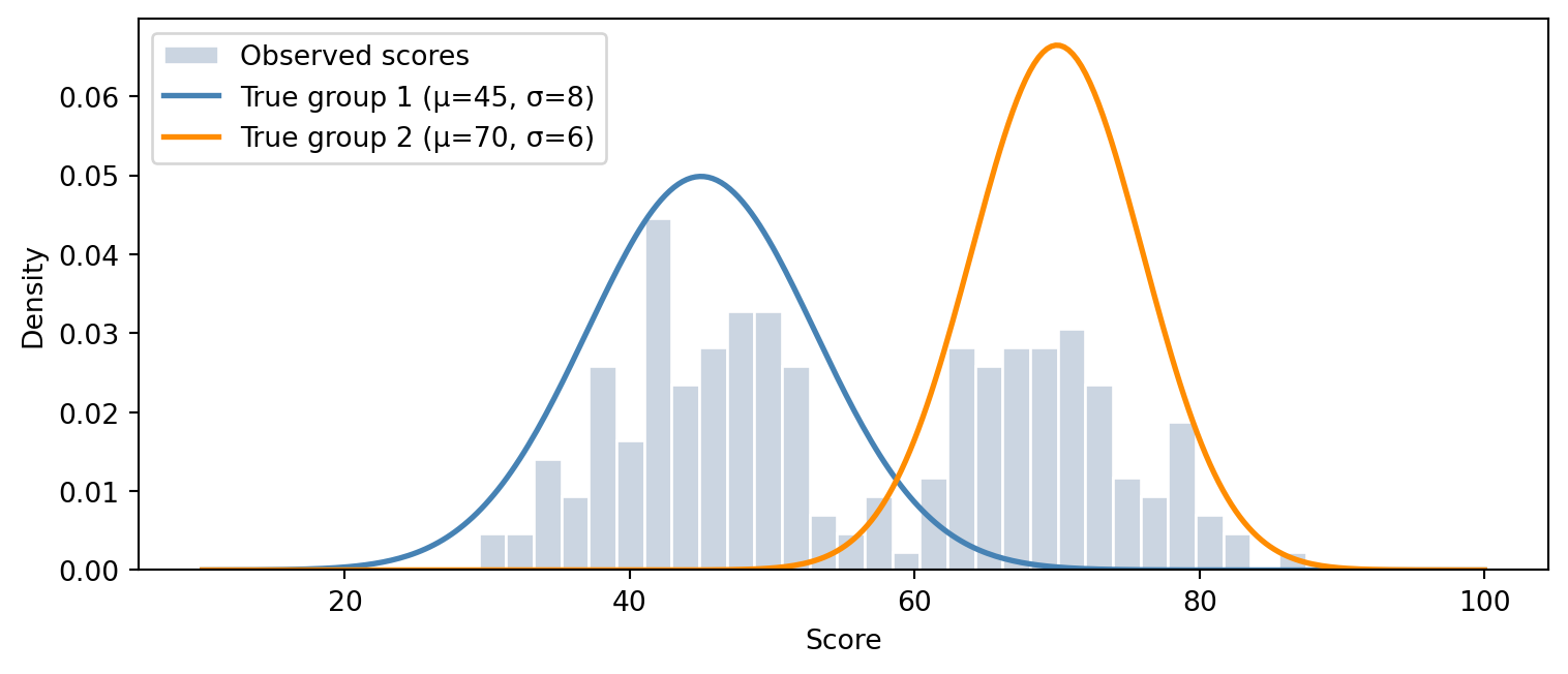
There are 220 exam scores in the dataset sampled from two overlapping Gaussian distributions. After sampling the exam scores, we shuffle the scores so that the algorithm can’t distinguish what scores come from what distribution. We include the original labels only for testing purposes to visualize how well the EM algorithm is able to find the correct labels. The EM algorithm follows roughly the following steps:
- Start with a rough guess at where the two groups are
- For each data point, calculate the probability it belongs to group 1 vs group 2
- Use those probabilities as soft weights to refit the distributions. Points clearly in one group pull hard on that group’s mean, uncertain points contribute a little to both
- After this we have slightly better distributions, which give slightly better probabilities next time
- Repeat until both stabilize
EM implementation
def em_gmm(X, K=2, n_iter=30, seed=0):
    rng_init = np.random.default_rng(seed)
    n = len(X)

    # --- Initialise parameters randomly ---
    mu    = rng_init.choice(X, K, replace=False)   # pick K random data points as starting means
    sigma = np.full(K, np.std(X))                  # same initial spread for all components
    pi    = np.ones(K) / K                          # equal mixing weights

    history = []   # store every snapshot for the OJS step-through

    for t in range(n_iter):

        # --- E-step: responsibilities ---
        # r[i, k] = p(z_i = k | x_i, theta^(t))
        r = np.array([
            pi[k] * norm.pdf(X, mu[k], sigma[k])
            for k in range(K)
        ]).T                              # shape: (n, K)
        r /= r.sum(axis=1, keepdims=True) # normalise rows

        # --- M-step: update parameters ---
        Nk    = r.sum(axis=0)
        mu    = (r * X[:, None]).sum(axis=0) / Nk
        sigma = np.sqrt((r * (X[:, None] - mu) ** 2).sum(axis=0) / Nk)
        pi    = Nk / n

        # --- Log-likelihood ---
        ll = np.log(
            sum(pi[k] * norm.pdf(X, mu[k], sigma[k]) for k in range(K))
        ).sum()

        history.append({
            "iter":  t + 1,
            "mu":    mu.tolist(),
            "sigma": sigma.tolist(),
            "pi":    pi.tolist(),
            "ll":    round(ll, 3),
            "r":     r.tolist(),   # full responsibility matrix. Used for rug colouring
        })

    return history


history = em_gmm(X, K=2, n_iter=30)

# Bridge to OJS
ojs_define(
    history     = history,
    X_data      = X.tolist(),
    true_labels = true_labels.tolist(),
    true_mu     = [45.0, 70.0],
    true_sigma  = [8.0,  6.0],
)
Interactive visualizer
The slider steps through the iterations of the EM algorithm. The top plot shows how the two Gaussians converge towards the most likely parameter values. The bottom plot shows the log-likelihood.
The two curves are the fitted Gaussians and the rug marks show each data point coloured by its soft assignment (blue = component 1, orange = component 2, yellow = uncertain). Grey dashed lines are the true means.
Log-likelihood across iterations. It can only ever increase.
References
[1]
C. M. Bishop, Pattern recognition and machine learning. Springer, 2006.